How We Built 300,000 Statistically Accurate Personas

The statistics behind Ditto's synthetic research panel — and where the model's honest limits lie.

There's something mildly absurd about claiming you've built 300,000 synthetic Americans. It sounds like the premise of a Philip K. Dick novel — or, worse, a startup pitch deck that's lost contact with reality.

And yet here we are.

At Ditto, our US persona model comprises 300,000 AI agents, each with a coherent demographic profile: age, sex, race, education, occupation, income, household composition, housing tenure, commute mode, healthcare coverage, religion, personality traits, and a name that reflects their ethnic and generational background. These agents participate in market research studies, answering questions with the specificity of real focus group participants.

The obvious question is: how closely do these 300,000 personas actually match the US population?

This is not a marketing claim. It's a statistical question with a statistical answer. What follows is a transparent account of the methodology, the calibration results, and — critically — the honest limitations.

Starting with the Gold Standard: Census Microdata

Every persona in our US model begins life as a record in the American Community Survey Public Use Microdata Sample (ACS PUMS), published annually by the US Census Bureau.

This is not a minor data source. The ACS PUMS is, for practical purposes, the authoritative dataset on who Americans are and how they live. It contains approximately 3.2 million individual records from the 2023 1-Year survey, each weighted to represent a proportional slice of the roughly 330 million civilians in the US non-institutional population. It is the same source used by government agencies, academic researchers, and major polling organisations to calibrate their own models.

From each PUMS record, we extract a comprehensive demographic profile: age, sex, race and ethnicity (using SPD-15 classifications), educational attainment, employment status, occupation (SOC major groups), industry (NAICS sectors), personal and household income, marital status, number of children, housing tenure, commute mode, internet access, healthcare coverage, disability and veteran status, citizenship, and language spoken at home.

We also join person-level records with their corresponding household records, linking individuals to household characteristics like household income, household size, and property tenure. The joining is done on the SERIALNO key — each person inherits the attributes of the household in which they reside.

The point worth emphasising: these are real, observed demographic combinations. A 34-year-old Hispanic woman who works as a dental hygienist in suburban Phoenix, rents her flat, has two children, earns $52,000, and takes the bus to work — that specific combination exists because a real person reported it to the Census Bureau. The downstream synthetic persona preserves these natural correlations, rather than assembling demographics independently (which would produce statistically plausible but ecologically implausible combinations).

From 3.2 Million to 300,000: Probability-Proportional Sampling

We don't use all 3.2 million PUMS records. We draw a sample of 300,000 using probability-proportional-to-size (PPS) sampling without replacement.

What this means in practice: each PUMS record has a person weight (PWGTP) assigned by the Census Bureau, reflecting how many people in the US population that record represents. Records representing more common demographic profiles have higher weights and are correspondingly more likely to be selected. A record with weight 850 (representing 850 people) is roughly 8.5 times more likely to be drawn than a record with weight 100.

This is deliberately not simple random sampling. PPS sampling produces a more representative initial draw because it respects the population structure embedded in the weights. The result is an approximately representative sample — but "approximately" is doing some work in that sentence, which is where calibration comes in.

The sampling fraction is approximately 9.4% of the PUMS universe (300,000 from 3.2 million). This is generous. For context, the Current Population Survey — the gold standard for US labour force statistics — uses roughly 60,000 households. Our initial draw is 5x larger.

The Raking Engine: Iterative Proportional Fitting

The sampled 300,000 records are then calibrated using iterative proportional fitting (IPF), more commonly known as raking. This is the same calibration method used by the Census Bureau, Pew Research Centre, Gallup, and essentially every serious survey organisation on the planet.

Here's what raking does. You specify a set of "control margins" — known population distributions that your sample must match. The algorithm then iteratively adjusts the weight of each record, nudging the sample's distributions towards the targets until convergence.

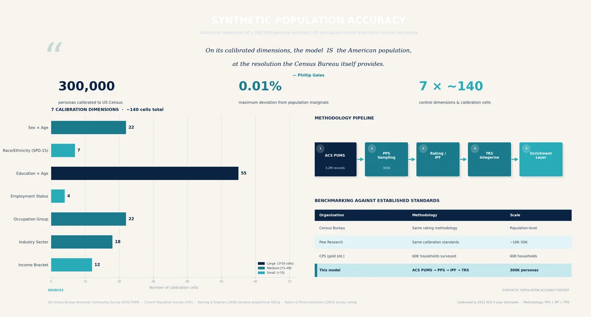
Our production configuration rakes to seven control margins, comprising approximately 140 individual cells:

The targets for each margin are computed by summing the PWGTP weights across the complete PUMS dataset, which gives us the Census Bureau's own estimate of the true US population distribution. These are authoritative numbers.

The raking converges when no single cell's adjustment ratio deviates from 1.0 by more than 0.01% — a tolerance of 1×10⁻⁴. In practice, convergence typically occurs within 10-15 iterations. At 300,000 records with 140 constraints, the system is heavily over-determined, and convergence is effectively guaranteed.

Several safeguards prevent instability. Individual weight adjustments are capped at 10× in either direction. Weight floors of 1×10⁻¹² prevent collapse to zero. The total weight is renormalised to the target sample size after each iteration.

After raking, the continuous weights are converted to integer clone counts via Truncated Replicate Sampling (TRS), which preserves the calibrated distribution while producing an exact headcount of 300,000. A record with calibrated weight 2.7 will appear either 2 or 3 times in the final population, with probability proportional to the fractional residual.

What This Means in Plain English

The national marginal distributions of our 300,000 personas match the US Census to within 0.01% across all seven calibrated dimensions.

That's worth sitting with for a moment. If the Census Bureau says 13.7% of the US population is aged 65-74 and female, our model will contain almost exactly 13.7% personas matching that description. If 4.2% of the population works in healthcare support occupations, our model will contain almost exactly 4.2% healthcare support workers.

This isn't an estimate or an aspiration. It's a mathematical consequence of the raking procedure. The algorithm does not stop until these margins match.

But calibrated marginals are only part of the story. What makes the model substantially richer than its explicit constraints is the correlation structure inherited from the microdata.

Because each persona originates from a real PUMS record — a real person's reported demographics — all the natural correlations between variables are preserved. Education correlates with income. Occupation correlates with industry. Race correlates with geography. Age correlates with disability status. These relationships aren't modelled or assumed; they're empirically observed and carried through.

This matters enormously for research fidelity. A model that independently assigns demographics would produce personas that are individually plausible but collectively incoherent — the demographic equivalent of an AI-generated face with six fingers. Our approach avoids this by construction.

Beyond Demographics: The Enrichment Layer

Demographics are the skeleton. The enrichment layer adds flesh.

Names are assigned using a weighted blend of three data sources: the Social Security Administration's national baby name data (selected by birth year matching the persona's age), New York City's baby name data (which uniquely provides name frequencies by mother's ethnicity), and the 2010 Census surname list (which provides surname frequencies by race). First names are weighted 30% SSA national / 70% NYC ethnicity-specific. Surnames are sampled with probability proportional to the persona's ethnic background. The result: a 52-year-old Black woman in Atlanta is far more likely to be named "Patricia Williams" than "Astrid Lindqvist."

Personality is modelled using the Big Five (OCEAN) framework. We generate correlated multivariate normal draws using Cholesky decomposition of published cross-trait correlation matrices, then apply demographic adjustments derived from the psychological literature: age effects (younger adults score higher on Openness and Neuroticism), gender effects (women score higher on Agreeableness), education effects (graduates score higher on Openness), and regional effects tuned for US macro-regions, Canadian provinces, German Bundesländer, and UK NUTS1 regions.

Religion is assigned probabilistically using national shares (Pew Research Centre data) with ethnicity-conditioned adjustments — Hispanic personas receive a Catholic probability boost; Black personas receive a Black Protestant boost; Asian personas receive Buddhist and Hindu boosts. The adjustments are mild (1.05–1.6× multipliers, renormalised), improving face validity without overriding the base distribution.

Income above the 95th percentile receives a Pareto tail adjustment. The ACS PUMS top-codes income at approximately $800K–1.1M, compressing the upper tail. We fit a Pareto distribution and replace the flat top-coded values with a more realistic heavy-tailed distribution. This matters for studies involving premium consumers, luxury brands, or high-net-worth segments.

The Honest Limitations

Transparency demands candour about where the model is weaker. Here are the principal limitations, in order of significance.

Religion lacks geographic variation. Our assignment uses national-level shares with ethnicity nudges, but does not incorporate state-level data. In practice, this means Utah receives approximately 2% LDS personas (the national average) when the true figure is closer to 60%. The Bible Belt receives roughly 24% Evangelical Protestant personas rather than the 40–50% that characterises much of the South. The architecture supports geographic conditioning — we simply haven't wired in the state-level data yet.

No state-level calibration. The raking operates at the national level. While the PPS sampling produces approximately correct state proportions, small states will have noisy distributions. Wyoming, with an expected ~500 personas, will show ±10% variation on key marginals. California, with ~35,000, will be within ±1%. Adding state as a raking margin is a straightforward improvement on the roadmap.

Voter registration is a crude model. Our current assignment uses a logistic-style function of age and education, producing plausible aggregate rates (~65–70% for eligible adults). However, it omits race/ethnicity effects, state-level variation, and — critically — party affiliation. For political research, this is the weakest component of the model.

The MENA gap. The SPD-15 race/ethnicity classification we use does not implement the MENA (Middle Eastern and North African) category that the new OMB standard introduces. MENA individuals (approximately 1–2% of the US population) are currently classified as White or "Some other race."

High incomes are synthetic above P95. The Pareto tail mapping produces a realistic distribution shape, but the specific dollar amounts above the 95th percentile are modelled, not observed. This affects approximately 15,000 personas.

How This Compares to Industry Standards

The overall approach — census microdata as a sampling frame, PPS sampling, raking to known marginals, TRS integerisation — is textbook survey methodology. It follows the same paradigm used by:

• RTI International's SynPUF (synthetic Medicare beneficiary data)

• The Census Bureau's own synthetic data products

• Pew Research Centre's American Trends Panel calibration

• The World Bank's microsimulation models

At N=300,000, the model is substantially larger than most survey-based synthetic populations. For any analysis conditioning on 2–3 demographic variables simultaneously, expected cell sizes are typically 100+ records — comfortably sufficient for stable estimates. Even the rarest control cells (85+ females, or Farming/Fishing/Forestry occupations) contain hundreds of personas.

The raking residual (the deviation between achieved and target marginals) is less than 0.01% per cell. The TRS integerisation introduces approximately 0.05% additional noise. These are well within acceptable tolerances for any reasonable application.

Conclusion

Our 300,000-persona US model is not an approximation of the American population. On its calibrated dimensions — sex, age, race, education, employment, occupation, industry, and income — it is the American population, at the resolution that the Census Bureau itself provides.

The uncalibrated dimensions (religion, voter registration, personality) are informed by credible data sources but carry wider margins. We've been deliberately transparent about these gaps, because we think the most persuasive thing a synthetic research platform can do is tell you exactly where its confidence ends.

The model gets better continuously. Geographic religion conditioning, state-level raking, MENA classification, and party affiliation are all on the roadmap. Each improvement is a data-wiring exercise, not an architectural change — the infrastructure already supports it.

In the meantime: if you're running consumer research with Ditto's US panel, you can be confident that the demographic composition of your research group matches the American population with a precision that would satisfy a Census Bureau methodologist.

Which is, admittedly, a rather odd sentence to write about synthetic humans. But here we are.